The SIR model is the classical mathematical tool to study the spread of an infectious disease like the current COVID-19 pandemic. In an SIR model, the population is divided into compartments of susceptible, infected and recovered individuals. A slight variation is the SIRD model, which has a fourth compartment for deceased individuals.
If $s(t)$, $i(t)$, $r(t)$ and $d(t)$ denote the fraction of the population of susceptible, infected, recovered and deceased individuals, the SIRD model comprises four ODEs,
$ds/dt = -\beta si$,
$di/dt = \beta si -\gamma i -\mu i$,
$dr/dt =\gamma i$,
$dd/dt = \mu i$,
where $s(t) + i(t) + r(t) + d(t) = 1$ at all times $t$.
One hypotheses underlying the SIRD model is that contacts between individuals occur randomly and that a contact between a susceptible and an infected individual has a certain probability of causing the susceptible to become infected. This hypothesis is reasonable with COVID-19, especially in view of the large number of asymptomatic infected individuals. Another hypothesis is that a recovered individual is immune to the disease, something that is still unknown for COVID-19 at the time of this writing.
An epidemic starts only if $di/dt$ takes positive values—that is, if $s> (\gamma +\mu)/\beta$. This can occur for large $s$ only if $R_0 = \beta/(\gamma+\mu) >1$; $R_0$ is the famous \emph{basic reproduction ratio}. The epidemic then proceeds in stages: a first stage of exponential growth of the fraction of infected individuals; a second stage, where the rate of new infections is almost constant; and a third stage, where the rate of new infections becomes negative and the epidemic becomes extinct.
Indeed, as soon as $s(t)$ has decreased to $1/R_0$, then $di/dt < 0$ and the epidemic disappears before the whole population has been infected. This is what is called group or herd immunity. Moreover, the fraction of infected individuals shows a peak.
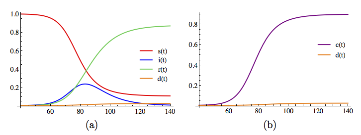
In practice, the data are not reliable, and it is very difficult to have access to the precise number of infected individuals. What we usually see is the cumulative curve of cases, $c(t)=i(t)+r(t)+d(t)$; see Figure~(b).
However, the official numbers underestimate the actual numbers because of unreported and asymptomatic cases; hence, the “official” cumulative curve of reported cases is below $c(t)$. Nonetheless, if we hypothesize that the number of reported cases depends roughly linearly on the cumulative cases, the official curve shows the three phases of the epidemic. Public health officials refer to the third stage as the flattening of the curve.
In the COVID-19 pandemic, the confinement policy (stay-at-home) abruptly changed the values of the parameters, transforming the initial system into one with $R_0<1$. Indeed, no national health system could have afforded 23\% of the population being simultaneously infected. But, with only a very small portion of the population having been infected, we are very far from group immunity, and any policy of “opening up” may bring $R_0$ back to a value greater than 1. To be continued …