Nick Tanushev, Chief Scientist, Z-Terra, Inc.
Like most animals, we have passive sensors that let us observe the world around us. Our eyes let us see light scattered by objects, our ears let us hear sound that is emitted around us and our skin lets us feel warmth. However, we rely on something to generate light, sound or heat for us to observe. One animal that is an exception to this is the bat. Bats use echolocation for navigation and finding prey. That is, they do not passively listen for sound, they actively generate sound pulses and listen for what comes back to figure out where they are and what’s for lunch.
From an applied mathematical point of view, active sensing using waves is a complex process. Waves generated by the active source have to be modeled as they propagate to an object, reflect and then arrive back at the receiver. Using the amplitude, phase, time lag and possibly other properties of the waves, we have to make inferences about the location of the object that reflected the waves and its properties. It is logical at this moment to ask “Well, if it is such a complex task, how can bats do it so easily?” The answer is that bats use a simplified model of wave propagation. In nearly constant media, such as air, high frequency waves propagate is straight lines and determining the distance between the bat and the object is simply a matter of the time it takes to hear the echo back and the speed of wave propagation. Our brain also uses the same trick to process what our eyes are seeing. You can easily convince yourself with an old elementary school trick: Put a pencil in a clear glass of water so that half of it is submerged and lean the pencil on the side so that it is not completely vertical. Looking from the side, it looks as if that the pencil is broken at the air water interface. Of course, this is an optical illusion because our brain assumes that light has traveled in a straight line when, in fact, it takes two different paths depending on whether it is propagating in the water or in the air.
A much more sophisticated version of echolocation is used by oil companies to image the subsurface of the earth. A classical description of the equipment used to collect data is a boat that has an active source (an air gun) and a set of receivers (hydrophones) that it drags behind it. The air gun generates waves, these waves propagate, reflect from structures in the earth and return to the hydrophones where they are recorded. The big difference is that seismic waves do not move along straight lines because the earth is composed of many different layers with varying composition. As a result the speed of propagation varies and waves take a complicated path through the earth.
Using the collected seismic data, an image of the subsurface is formed by starting with a rough estimate for the velocity, modelling the source forward in time and the receiver wave fields backward in time using the wave equation. The source and receiver wave fields are then cross correlated in time to produce an image of the earth. The mismatch between images formed from different source and receiver pairs can be used to get a better estimate of the velocity. The process is iterated to improve the velocity. Thus, the key to building a good model of the subsurface is being able to solve the wave equation quickly and accurately many times. Direct discretization of the wave equation is computationally too expensive and, like the bats, we have to find a simplified model of wave propagation which models the wave propagation to a good enough accuracy and can be solved rapidly. Asymptotic methods valid for high frequency waves are used to model the wave propagation. Seismic waves are not considered particularly high frequency, but “high frequency” really means that the wave length is small compared to the size of the simulation domain and the variations of the wave propagation speed and in this case both of these assumptions are valid.
The most commonly used method is based on geometric optics, also referred to as WKB or ray-tracing. The key idea is to represent the wave field using an amplitude function and a phase function. Usually, these functions are slowly varying (when compared to the wave oscillations) and can be represented numerically by far less points than the original wave field. However, there is no free lunch and this gain comes at the price that the partial differential equation for the phase function is non-linear. One major problem is that the equation for the phase can only be solved classically for short time and we have to use more exotic solutions such as viscosity solutions after that. This departure from a classical solution is an observable phenomenon called “caustic regions” and we have all observed them as the dancing bright spots at the bottom of a pool. At caustic regions, waves arrive in phase and can no longer be represented using a single phase functions.
More recently, an alternative method to geometric optics, called Gaussian beams, has gained popularity. Gaussian beams are asymptotic high frequency wave solutions to hyperbolic partial differential equation (such as the wave equation) that are concentrated on a single curve. Gaussian beams are a packed of waves that propagate coherently. An easy example to think about is a laser pointer. It forms a tight beam of light that is concentrated along a single line. Gaussian beams are essentially the same, except that the width of the beam is much smaller and in media with varying speed of wave propagation, the curves are not necessary a straight line. The amplitude of this coherent packet of waves decays like a Gaussian distribution and gives them their name. One of the most important features of Gaussian beams is that they remain regular for all time and do not breakdown at caustics. The trick to making Gaussian beams a useful tool for solving the wave equation is to recognize that since the wave equation is linear, we can take many different Gaussian beams and add them together and still obtain an approximate solution to the wave equation. Such superpositions of Gaussian beams allow us to approximate solutions that are not necessarily concentrated on a single curve. Since each Gaussian beam does not breakdown at a caustic, neither will their superposition.
The existence of Gaussian beam solutions has been know since the 1960s, first in connection with lasers. Later, they were used in pure mathematics to analyse the propagation of singularities in partial differential equations. Since the 1970s, Gaussian beams have been used sporadically in applied mathematics research with a major industrial success in imaging earth is sub-salt regions in the Gulf of Mexico in the mid 1980s. From a mathematics point of view, questions about the accuracy of Gaussian beam superposition solutions and the rate of convergence to the exact solution has only been answered in the last ten years, justifying the use of such solutions in numerical methods.
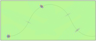 Single Gaussian beam: Several snap-shots of he real part of the wave field for a Gaussian beam are shown. Time flows along the plotted curve, which shows the path of the packet of waves.
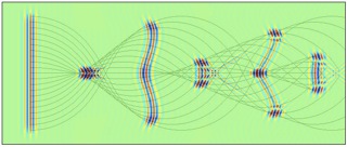 Gaussian beam superpositions: Several snap-shots of he real part of the wave field for a Gaussian beam superposition beam are shown. The plotted
lines are the curves for each Gaussian beam.
Note that the wave field remains regular at the caustics, where the curves cross
and traditional asymptotic methods breakdown.
Gaussian beam superpositions: Several snap-shots of he real part of the wave field for a Gaussian beam superposition beam are shown. The plotted
lines are the curves for each Gaussian beam.
Note that the wave field remains regular at the caustics, where the curves cross
and traditional asymptotic methods breakdown.