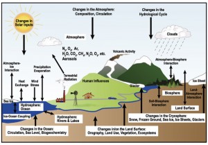
[Adapted from Chapter 1 of the forthcoming text “Mathematics and Climate” by Hans G. Kaper and Hans Engler, to be published by the Society for Industrial and Applied Mathematics (SIAM), 2013.]
What is the role of mathematics in climate science? Climate science, like meteorology, is largely a branch of physics; as such, it certainly uses the language of mathematics. But could mathematics provide more than the language for scientific discourse?
As mathematicians, we are used to setting up models for physical phenomena, usually in the form of equations. For example, we recognize the second-order differential equation $$L x ̈(t)+ g \sin x(t) = 0$$ as a model for the motion of a physical pendulum under the influence of gravity. Every symbol in the equation has its counterpart in the physical world. The quantity $x(t)$ stands for the angle between the arm of the pendulum and its rest position (straight down) at the time $t$, the constant $L$ is the length of the pendulum arm, and $g$ is gravitational acceleration. The mass of the bob turns out to be unimportant and therefore does not appear in the equation. The model is understood by all to be an approximation, and part of the modeling effort consists in outlining the assumptions that went into its formulation. For example, it is assumed that there is no friction in the pendulum joint, there is no air resistance, the arm of the pendulum is massless, and the pendulum bob is idealized to be a single point. Understanding these assumptions and the resulting limitations of the model is an essential part of the modeling effort. Note that the modeling assumptions can all be assessed by an expert who is not a mathematician: a clockmaker can estimate the effect of friction in the joint, the difficulty of making a slender pendulum arm, and the effort in making a bob that offers little air resistance. As mathematicians, we take the differential equation and apply the tools of the trade to extract information about the behavior of the physical pendulum. For example, we can find its period — which is important in the design of pendulum clocks — in terms of measurable quantities.
Would it be possible to develop a “mathematical model” of the Earth’s climate system in a similar fashion? Such a model should stay close to physical reality, climate scientists should be able to assess the assumptions, and mathematicians and computational scientists should be able to extract information from it.

The figure on the left gives a climate scientist’s view of the Earth’s climate system: a system with many components that interact with one another either directly or indirectly, and with many built-in feedback loops, both positive and negative. To develop a mathematical model of such a complex system, we would need to select variables that describe the state of the system (air temperature, humidity, fractions of aerosols and trace gases in the atmosphere, strength of ocean currents, rate of evaporation from vegetation cover, change in land use due to natural cycles and human activity, and many many more), take the rules that govern their evolution (laws of motion for gases and fluids, chemical reaction laws, land use and vegetation patterns, and many many more), and translate all this into the language of mathematics. It is not at all clear that this can be done equally well for all components of the system. The laws for airflow over a mountain range may be well known, but it is much harder to predict crop use and changes in vegetation. The ranges and limitations of any such model would remain subject to debate, much more so than in the case of the pendulum equation, and the resulting equations would likely cover several pages and would be far too unwieldy for a mathematical analysis. This would leave a computational approach as the only viable option. But even here we would face limitations, given the available computational resources and the scarcity of data.
Surprisingly often, mathematics can offer perspectives that complement or provide insight into the results of observations and large-scale computational experiments. Through inspired model reduction and sometimes just clever guessing, it is often possible to come up with relativity simple models for components of the climate system that still retain some essential features observed in the physical world, that reproduce complex phenomena quite faithfully, and that lead to additional questions. The two figures on the right illustrate a simple energy balance model for the entire planet. It posits that the solar energy reaching the Earth must balance the energy that the Earth radiates back into outer space; otherwise, the planet will heat up or cool down. The model focuses on the global mean surface temperature and reproduces the current state of the climate system remarkably well with just a few physical parameters (solar output, reflectivity of the Earth’s surface, greenhouse effect). The model also shows that the Earth’s climate system can have multiple stable equilibrium states. One of these states is the “Snowball Earth” state, where the entire planet is covered with snow and ice and temperatures are well below freezing everywhere. Why is the planet at today’s climate when much colder climates are also possible? Has the planet ever been in one of the much colder climate states in the past? (The answer is yes.) Is there any danger that Earth could again revert to a much colder climate in the future? How would this happen? Mathematics can raise these questions from a very simple climate model and also support or rule out certain answers using an analysis of the model.
